Mathematica
Introduction
s = Table[{0, n, m*GoldenRatio}, {n, -1, 1, 2}, {m, -1, 1, 2}];
s = Partition[Flatten[s], 3];
s = Append[s, {0, 0, 0}];
s = Union[s, Map[RotateRight, s], Map[RotateLeft, s]];
s = Graphics3D[Table[{Hue[Random[]], Sphere[s[[k]]]}, {k, 12}]]
Export["kissing.stl", S, "STL"]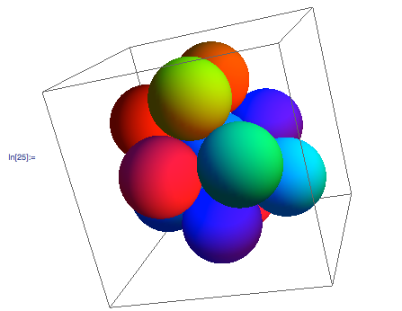
Artist and mathematician, George Hart taught a course in the Fall of 2007 at Stony Brook University that covered
procedural generation of three-dimensional forms, with an emphasis on making
triangulated manifold boundaries suitable for solid freeform fabrication (SFF).
Hart uses
Mathematica to generate his models.
Introduction to Mathematica
To start a new program in Mathematica, create a new
Notebook. A
Notebook is the main window for entering input and for displaying results
To enter input, just start typing. You can create, save, open and close a notebook using the
File menu.
Notebooks are organized into units called
cells. These cells are identified by the brackets on the right hand side.The
insertion point is indicated by a horizontal line that appears after your output; it is called the
cell insertion bar . This is where a new cell will appear after you start typing. Move the cursor in your notebook window until it becomes a horizontal I-beam.
To create a text cell, get a cell insertion bar. Then choose
Format >Style >Text or use the keyboard shortcut Alt+7 (Command+7 on Mac).
To evaluate input, press
SHIFT+ENTER.
Mathematica supports standard mathematical operations. In addition to using
* for multiplication, you can just separate numbers by a space. So
xy is not the same as
x y, but
x y is the same as
x*y
Calculations in Mathematica are done by calling functions. The most general way to enter a function is to give the name of the function followed by square brackets that enclose the argument or arguments of the function. If a function has more than one argument, separate them by commas. (Function arguments are enclosed in square brackets and are separated by commas.)
The function N is used to give numerical approximations to its first argument:
specifies that x = 0 to 20
{2, 4, 6} + {100, 40, 15}
returns {102,44,21}
Mathematica is case sensitive and the names of built-in functions are always capitalized.
Like other programming languages, you can assign values to variables like this:
If you need to check the value of your variable, do this:
Don't forget to
Clear your global variables when you are done with them:
A sequence of statements separated by semicolons is called a
compound expression. You can also nest statements.
The
Mathematica Documentation Center is the main interface to documentation in Mathematica. Open the documentation by going to the
Help menu in Mathematica and then selecting
Documentation Center. Alternatively, select a function name in any notebook and press F1 (or fn F1). Just like variables you can see a function definition by preceding the function with a
?
When looking up a function, you can use the
* symbol to represent a wildcard:
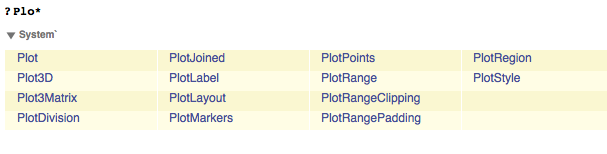
If you type a function and then press CTRL+SHIFT+K or Command+SHIFT+K, Mathematica will show you the parameters that the function takes.
Plot takes one parameter. To plot several functions together, you can put them in a list as the first argument to Plot:
Plot[{Sin[x], 2 Sin[2 x], 1/3 Sin[3 x]}, {x, 0, 2 Π}]
The Plot3D function plots a function as a three-dimensional surface.
Plot3D[Sin[x - Sin[y]], {x, 0, 3 Pi}, {y, 0, 4 Pi}]To rotate this graphic, move your cursor over the graphic, hold down the left mouse button, and rotate the image by moving the mouse.
To zoom in and out, hold down Command or Option Key and move your cursor over the graphic and then drag the pointer up to zoom in and down to zoom out.
Use the SHIFT key to pan.
You can combine surfaces:
Plot3D[{Sin[x - Sin[y]], Sin[y - Cos[x]]}, {x, 0, 3 Pi}, {y, 0,
  4 Pi}]
Procedural Generation
The following is from George Hart's
Procedural Generation of Sculptural Forms
Mathematica has a built in Polyhedra library which includes Platonics, Archimedeans, and their duals. The function
PolyhedronData[] takes a string and returns that type of polyhedron. It is returned in a form called a
graphics complex (GC) which displays the form as a resizable 3D image that can be rotated by dragging with the mouse:
PolyhedronData["Dodecahedron"]
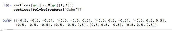
The GC format contains information about the shape that can be extracted. The xyz coordinates of the vertices of a GC are in the position subscripted as [[1,1]], so to extract them you would write:
vertices[gc_]:= N[gc[[1,1]]]
Mathematica’s syntax for defining functions is
:= and the underscore after the variable gc indicates that the argument of gc can be anything, not just the literal symbol gc.
The N[] function causes the result to be returned in a numeric (floating point) format, without symbolic expressions such as square roots.
The example below uses this function to find the vertices of the built-in cube and observe that it is an
axis-aligned unit-edge-length cube centered at the origin. The output, at right, is a list of eight points; each point is a list of the form {x,y,z}.
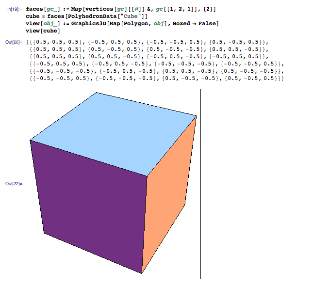
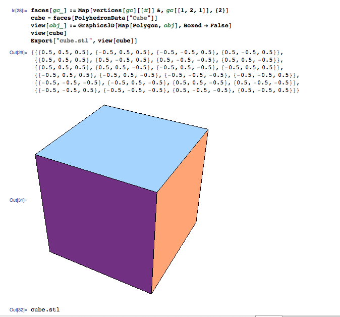
The faces of a GC can be extracted with an this conversion function:
faces[gc_] := Map[vertices[gc][[#]]&, gc[[1,2,1]],{2}]
Each face is a list of points recorded in counterclockwise order as seen from outside the object, so the list of faces is a list of lists of lists. The generality of the list data type is convenient because many built-in list operations can be used on lists with any type of content. However, be careful to keep track of what each list represents. Typing this assignment to the variable cube generates the six lines of output at right, which we understand to represent a cube as having six faces, each with four points:
faces[gc_] := Map[vertices[gc][[#]]&, gc[[1,2,1]],{2}]
cube = faces[PolyhedronData["Cube"]]
You'll can use this list-of-faces format without printing it out. Unlike a GC, it does not display as a mouse-rotatable polyhedron. So you need to write a viewing function which converts your list-of-faces format into a GC for display. Use an option to omit the default bounding box, which can be seen above around the dodecahedron. Then the
view command shows your polygon. In Mathematica, you can rotate it to see all sides:
To physically produce the objects convert your list-of-faces object into an .stl file:
Export["cube.stl", view[object]]
Tetrahedron and compounds
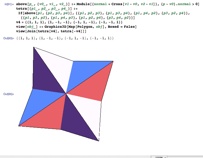
To distinguish an object's interior from it's exterior, Rapid Prototyping machines require that vertices of each face be listed in counterclockwise order. A function to create a tetrahedron from a list of four vertices determines this ordering from a single test of
aboveness, using Mathematica's
If [test, then, else] syntax:
above[p_, {v0_, v1_, v2_}] :=
 Module[{normal = Cross[v1 - v0, v2 - v1]}, (p - v0).normal > 0]
tetra[{p1_, p2_, p3_, p4_}] :=
 If[above[p1, {p2, p3, p4}], {{p1, p2, p3}, {p1, p3, p4}, {p1, p4,
    p2}, {p3, p2, p4}}, {{p1, p3, p2}, {p1, p4, p3}, {p1, p2,
    p4}, {p3, p4, p2}}]
v4 = {{1, 1, 1}, {1, -1, -1}, {-1, 1, -1}, {-1, -1, 1}}
view[obj_] := Graphics3D[Map[Polygon, obj], Boxed -> False]
view[tetra[v4]]
Here v4 is to be a list of four nonadjacent vertices of a cube so you can build a regular tetrahedron from them:
v4={{1,1,1},{1,-1,-1},{-1,1,-1},{-1,-1,1}} view[tetra[v4]]
The
Join function combines two lists into one. A minus sign applied to a list distributes to the elements of the list. So the following line produces the faces for the
Stella Octangula, i.e., the compound of two tetrahedra in a common cube. (Faces pass through each other, but this will build on most SFF machines.)
view[Join[tetra[v4], tetra[-v4]]]
Next you can create the uniform compound of five tetrahedra. Let v be the vertices of a regular dodecahedron. Five different subsets of four vertices are joined to give the following.
v=vertices[PolyhedronData["Dodecahedron"]]
view[Join[tetra[{v[[1]],v[[11]],v[[17]],v[[20]]}], tetra[{v[[2]],v[[4]],v[[7]],v[[9]]}],
tetra[{v[[3]],v[[12]],v[[13]],v[[15]]}], tetra[{v[[5]],v[[8]],v[[14]],v[[18]]}], tetra[{v[[6]],v[[10]],v[[16]],v[[19]]}]]]
Transformations: translate, scale, and rotate
You can translate an object by adding a vector offset to each vertex. The syntax used here is a bit cryptic, with Map used to create a list by applying a function to elements of a given list, the
& symbol is used to create an anonymous function with
# as the argument placeholder, and
{2} as a special argument to Map indicating the function is to be applied at
level 2 (the xyz points) rather than to the top level elements of the list (the faces). Test the function by creating a cube with another cube translated 1.1 units in the X direction:
translate[obj_, offset_]:= Map[(#+offset)&, obj, {2}]
view[Join[cube, translate[cube,{1.1,0,0}]]]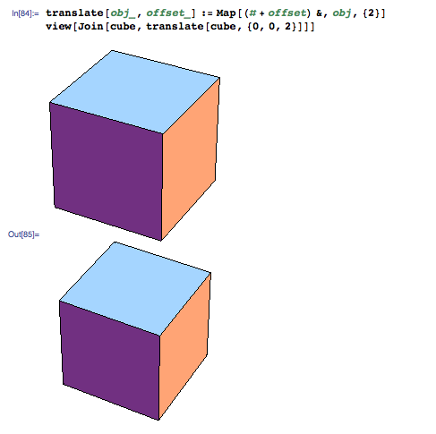
Scale an object by multiplying it by a scale factor. Multiplication of a scalar times a list distributes into the list, so eventually percolates down to the individual X, Y, and Z coordinates of the points in the faces in the object. Note that an
* is not required to indicate multiplication in Mathematica's syntax; a space also works. The following generates a unit cube and a translation of a half-size cube:
view[Join[cube, translate[0.5 cube, {0.75,0,0}]]]
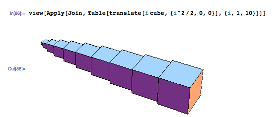
The syntax for creating the list {f[1], f[2], ..., f[10]} is Table[f[i], {i, 1, 10}].
You can create ten-layers of joining cubes of size 1 through size 10, like this
view[Apply[Join, Table[translate[i cube,{i^2/2,0,0}], {i,1,10}]]]
You can rotate an object by multiplying its vertex coordinates by a rotation matrix. There is a built-in function that creates the rotation matrix corresponding to a given angle and rotation axis (Escher’s Waterfall):
rotate[obj_, angle_, axis_] := Map[(RotationMatrix[angle,axis].#)&, obj, {2}]
view[Join[rotate[cube, Pi/4, {1,0,0}],
rotate[cube, Pi/4, {0,1,0}],
rotate[cube, Pi/4, {0,0,1}]]]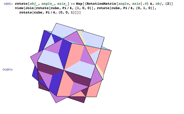
Manipulating
Manipulate lets you create interactive applications.
The output you get from evaluating a Manipulate command is an interactive object containing one or more controls (sliders, etc.) that you can use to vary the value of one or more parameters. The output is not just a static result, but is a running program you can interact with.
The code below allows the user to change the value of
a from 0 to 2.
Manipulate[Plot[Sin[x (1 + a x)], {x, 0, 6}], {a, 0, 2}]
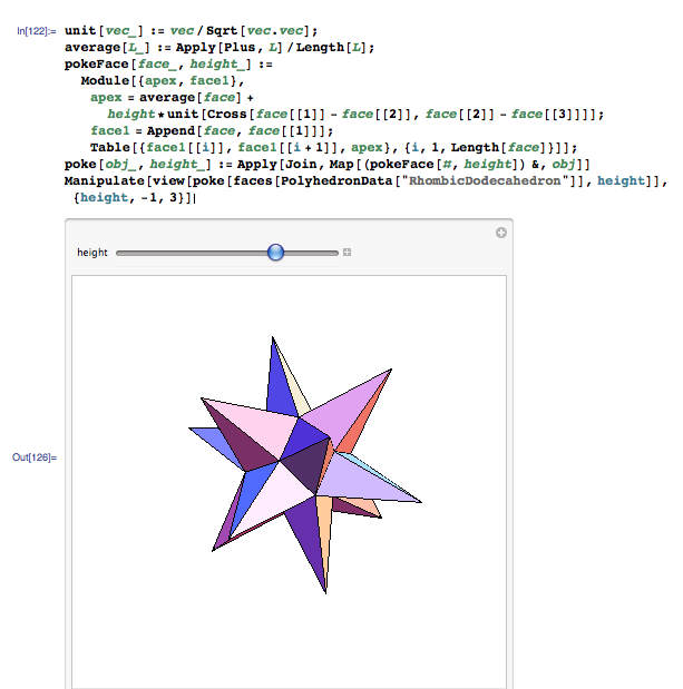
This line of code changes the poke height
view[obj_] := Graphics3D[Map[Polygon, obj], Boxed -> False];
vertices[gc_] := N[gc[[1, 1]]]
faces[gc_] := Map[vertices[gc][[#]] &, gc[[1, 2, 1]], {2}];
unit[vec_] := vec/Sqrt[vec.vec]
average[L_] := Apply[Plus, L]/Length[L]
pokeFace[face_, height_] :=
  Module[{apex, face1},
   apex = average[face] +
     height*unit[
       Cross[face[[1]] - face[[2]], face[[2]] - face[[3]]]];
   face1 = Append[face, face[[1]]];
   Table[{face1[[i]], face1[[i + 1]], apex}, {i, 1, Length[face]}]];
poke[obj_, height_] := Apply[Join, Map[(pokeFace[#, height]) &, obj]]

Manipulate[
 view[poke[faces[PolyhedronData["RhombicDodecahedron"]],
   height]], {height, -1, 3}]
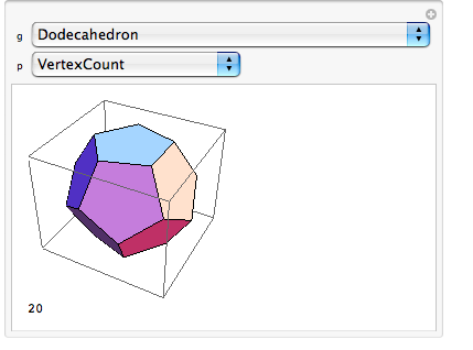
Manipulate[
 Column[{PolyhedronData[g], PolyhedronData[g, p]}],
 {g, PolyhedronData[All]},
  {p, Complement @@ PolyhedronData /@ {"Properties", "Classes"}}]
In the above example g will be all the types of PolyhedronData and p will be all the Properties. The display will show the polyhedron above the property:
To export it, click on the + sign, get a snapshop and re-write it:
g = "AcuteGoldenRhombohedron"
shape := PolyhedronData[g]
View[shape]
Export["poly.stl", shape]
Exporting DXF
If you want to explore fractals, you can export the images as .dxf files and then open them up in OpenSCAD and linear_extrude() them.
Fractals
A fractal is a mathematical object that is repeated at ever smaller or larger scales sto produce irregular shapes that could never be represented by Euclidian Geometry.
//Introduction
You can connect Arduino to Mathematica using the Serial Call and Response concept.
William J Turkel does computational history, big history, STS, physical computing, desktop fabrication and electronics. He created a small guide to connecting the Arduino to Mathematica on Mac OS X with SerialIO in December of 2011:
A Simple Circuit
Create a simple circuit with a potentiometer and an Arduino board connected to a computer via a USB cable.
- Connect the potentiometer to pin A0 on the Arduino
-
Copy and upload the following code into Arduino:
  //----------------------Arduino code-------------------------

/*
 arduino_mathematica_example

 This code is adapted from
 http://arduino.cc/en/Tutorial/SerialCallResponse

 When started, the Arduino sends an ASCII A on the serial port until
 it receives a signal from the computer. It then reads Analog 1,
 sends a single byte on the serial port and waits for another signal
 from the computer.

 Test it with a potentiometer on A1.
 */

int sensor = 0;
int inByte = 0;

void setup() {
  Serial.begin(9600);
  establishContact();
}

void loop() {
  if (Serial.available() > 0) {
    inByte = Serial.read();
    // divide sensor value by 4 to return a single byte 0-255
    sensor = analogRead(A0);
    sensor=map(sensor, 0,1024, 0,255);
    delay(15);
    Serial.write(sensor);
  }
}

void establishContact() {
  while (Serial.available() <= 0) {
    Serial.print('A');
    delay(100);
  }
}
//--end Arduino code--------------------------------
- Upload the sketch to the Arduino. Close the Arduino IDE (otherwise the device will look busy when you try to interact with it from Mathematica).
- Install the SerialIO package in /HD/Library/Mathematica/Applications
and make sure that it is in your path. If the following command does not evaluate to True
MemberQ[$Path, "/Library/Mathematica/Applications"]
AppendTo[$Path, "/Library/Mathematica/Applications"]
- Edit the file
/Library/Mathematica/Applications/SerialIO/Kernal/init.m
so the line
$Link = Install["SerialIO"]
$Link =
Install["/Library/Mathematica/Applications/SerialIO/MacOSX/SerialIO",
LinkProtocol -> "Pipes"]
-
If you need to find the port name for your Arduino, you can open a terminal and type
-
Paste the following into a notebook:
<<SerialIO`

myArduino = SerialOpen["/dev/tty.usbmodem3a21"]

SerialSetOptions[myArduino, "BaudRate" -> 9600]

SerialReadyQ[myArduino]

Slider[
 Dynamic[Refresh[SerialWrite[myArduino, "B"];
  First[SerialRead[myArduino] // ToCharacterCode],
  UpdateInterval -> 0.1]], {0, 255}]
- The Mathematica code loads the SerialIO package, sets the rate of the serial connection to 9600 baud to match the Arduino, and then polls the Arduino ten times per second to get the state of the potentiometer. It doesn’t matter what character you send the Arduino (here we use an ASCII B). You need to use ToCharacterCode[] to convert the response to an integer between 0 and 255. If everything worked correctly, you should see the slider wiggle back and forth in Mathematica as you turn the potentiometer. When you are finished experimenting, you need to close the serial link to the Arduino with:
New York State Learning Standards
