Introduction

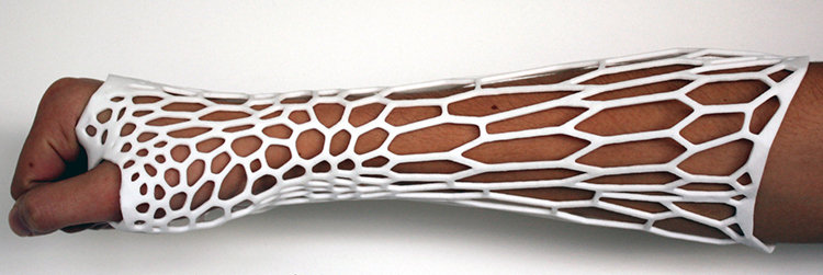Image from project2gether.com	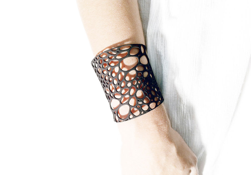Image from thingfuture.com
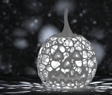
Image from 3dsoup.com	© 3Dizingof.com Image from Adafruit
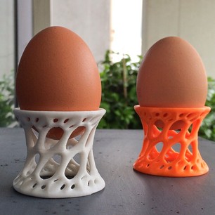
Image from ink361.com

A Dirichlet tessellation, or Voronoi diagram, is a partitioning of a plane containing a set of points into convex polygons such that

• each polygon contains exactly one generating point
• every point in a given polygon is closer to its generating point than to any other

The individual cells resulting from this process are known as Dirichlet regions, Thiessen polytopes, or Voronoi polygons.

Voronoi diagrams were considered as early as 1644 by René Descartes and were used in 1850 by Lejeune Dirichlet in the investigation of positive quadratic forms. They were also studied by Georgy Voronoi in 1907. Voronoi diagrams find widespread applications in areas such as computer graphics, epidemiology, geophysics, and meteorology. A particularly notable use of Voronoi diagrams is the analysis of the 1854 Cholera epidemic in London, in which physician John Snow determined a strong correlation between death rates and proximity to the infected Broad Street water pump.

(Wolfram)

Voronoi diagrams have a wide range of uses from calculating the area per tree in the forest, to determining the source of Cholera. In general these diagrams are useful for finding "who is closest to whom." Voronoi diagrams are used:

• Path planning in the presence of obstacles
• Model and analyze plant competition
• Analyzing patterns of urban settlements
• Geometric modeling
• Closest pairs algorithms
• Nearest-neighbor queries

Given a set of points, a Voronoi diagram defines a series of cells surrounding each point. Each cell contains all points that are closer to its defining point than to any other point in the set. As a result the "borders" of the cells are equidistant between the defining points of the adjacent cells.

Say you have a map of your city, and on it you have located a set of points representing every fast food restaurant. Creating a Voronoi diagram from these points would enable you (on your walk through the city) to know which restaurant you're closest to at any given time. Of course, an application that simple could be solved more efficiently via other methods, but let's raise the stakes a bit. What if you want to know the percentage of your walk that will be closest to one particular McDonalds. Suddenly, without a Voronoi diagram, this is tricky. With a Voronoi diagram, however, it's a simple matter of intersecting the line that represents your walk with the cell that surrounds that particular restaurant.

Voronoi diagrams can also be used to make maps, not just analyze them. Say you have a set of points that represent air quality sample locations. To quickly generalize the sample points into a local map… bam! Voronoi diagram!

Don Havey

How to Draw A Voronoi Cell

First way: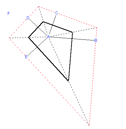

Image frommathforum.org

Start with a figure of six points ABCDE (F comes later). To construct the Voronoi cell of A draw the perpendicular bisectors of segments AB, AC, AD, and AE. These perpendicular bisectors enclose a polygon around point A. In the figure above this polygon is the bold black quadrilateral. Only the sides of this polygon form the cell around A. The rest can be removed (as is done in the figure).
from Second way:

1. Input Sites.
2. Connect Nearest Neighbors (shortest line wins).
3. Find Center Points.
4. Draw Perpendicular Bisectors.
5. Trace Cells.

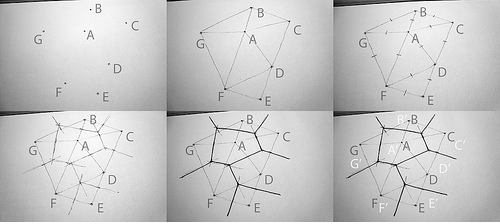
Images from sevensixfive

Use different colors for the input sites, the Delauney lines, and the bisectors.

1. The input points, step one, are called sites, labeled here A, B, C, etc.
2. Connect the sites to all of their nearest neighbors without making a line that crosses another. This is known technically as the Delauney Triangulation.
3. Find and mark the centerpoint of every line on the Delauney graph.
4. Draw the perpendicular bisector for each Delauney line. This is where careful accuracy, in finding the centerpoints, and in drawing a tight 90 degree angle, pays off. If everything has been done correctly, there will always be three lines converging at a point, unless the input sites are on a perfectly regular rectangular grid.
5. Retrace the outline of each Voronoi cell from the perpendicular bisectors. There will be one cell for every site, and at the end, each cell is just the set of all surface area points that are closer to its site than any of the other sites, as illustrated in the last panel: A' -> A, B' -> B, etc.

Lesson Purpose

• To explore voronoi cells.
• To create art with math.

Materials

• 3D printer
• Access to the internet.
• Applications: MeshLab, Blender, TinkerCad

Resources

• Wolfram MathWorld
• Wolfram Demonstration Project
• Voronoi Diagrams: Applications from Archaology to Zoology
• zheng3's Meshlab tutorial
• sevensixfiveLHow to: Draw the Voronoi Diagram
• codeproject: Create a Voronoi Diagram
• Mesh—A Processing Library
• Don Havey's Voronoi Diagram tutorial
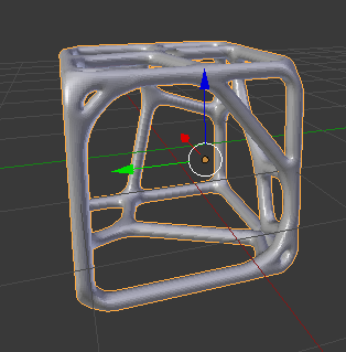
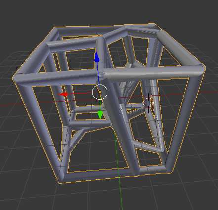
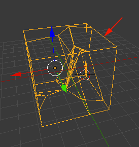
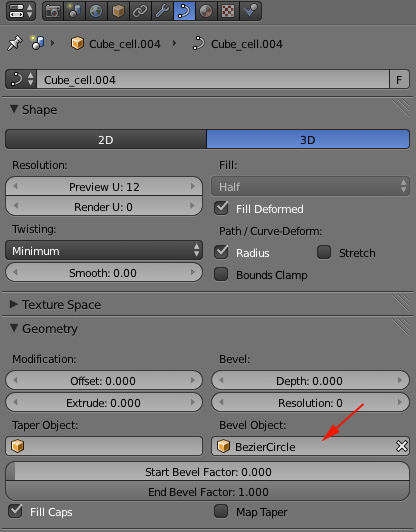
• Voronoi Encapsulation, Walk Through (How to) using Blender & 3D Printing the result Gareth Chiprobot

Procedure

1. Open MeshLab
2. Import or add a new form:Filters>Create New Mesh Layer>some_form
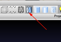
3. Turn on flat lines
   
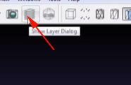
4. Enable Layers. This will bring up the Layers sidebar.
   
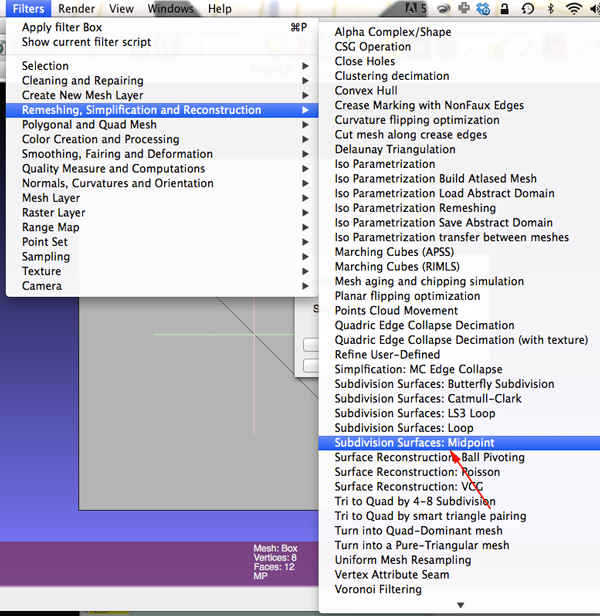
5. You want around 300k faces so select Filter>Remeshing>Subdivision surfaces:Loop or midpoint.
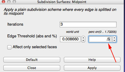
6. Change the perc field to .5
   
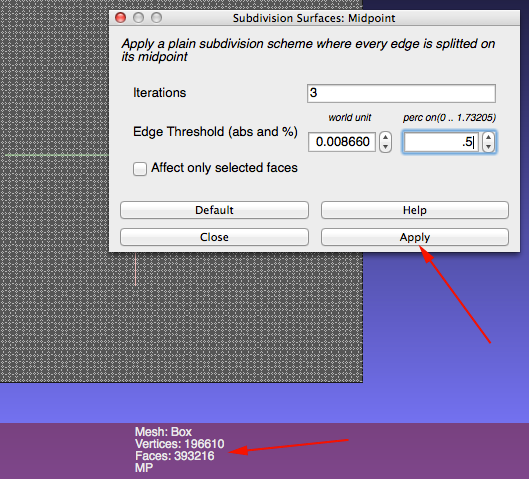
7. Keep clicking on Apply until you get close to 300k faces
   
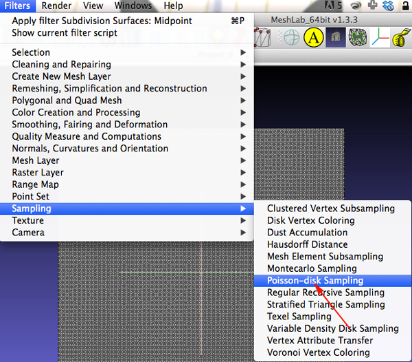
8. Select Filter>Sampling>Poisson Disk Sampling
   
9. In the dialog box enter 35
   
   
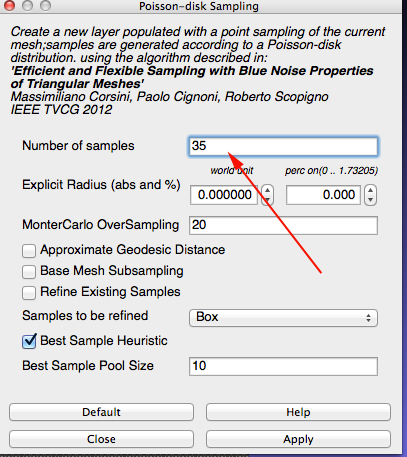
   You are looking for about 50 points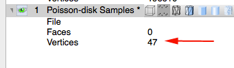
   
   
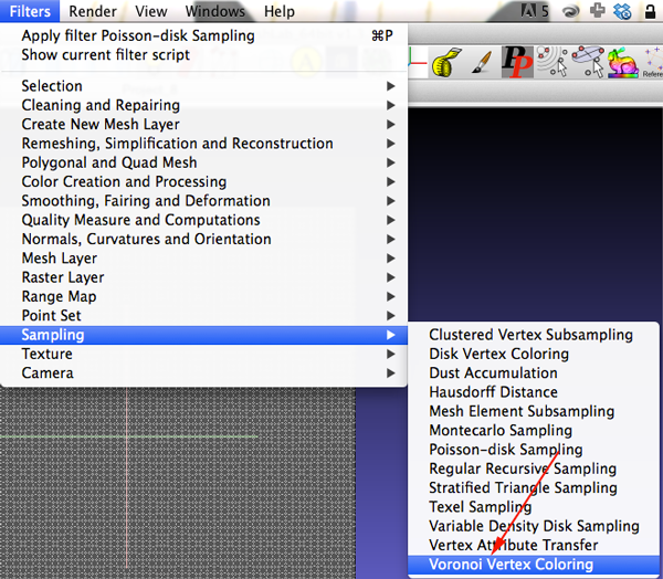
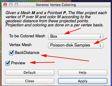
   The points represent your sites
10. Select Filter>Sampling>Voronoi Vertex Coloring
    
11. Make sure your dialog box is set up similar to the one below:
    
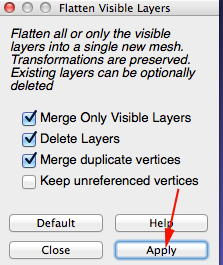
12. CTRL+click on the top layer and select Flatten Visible Layers
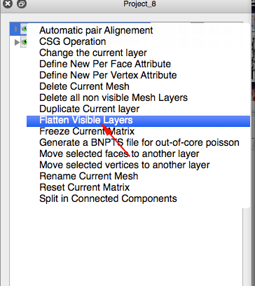
13. Apply flatten
    
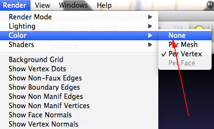
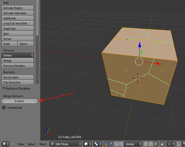
14. Remove the interior faces. First click on Render>Color>None
    
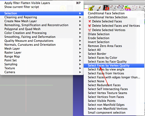
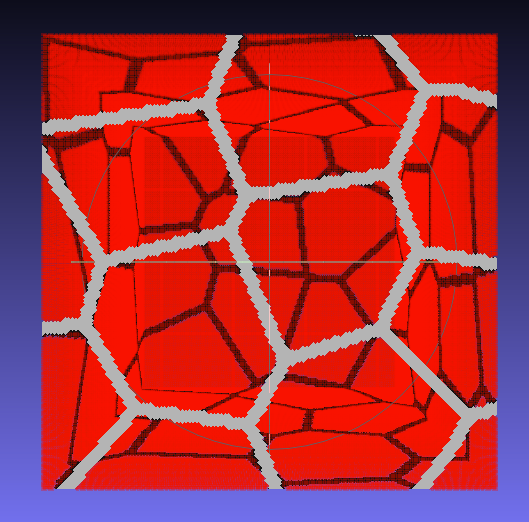
15. Select Filters>Selection>Select Faces by Vertex Quality
    
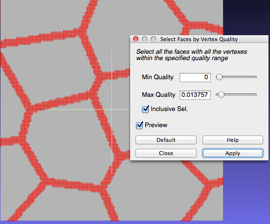
16. Check the Preview checkbox and adjust the sliders
    
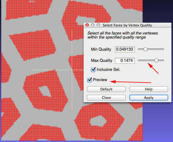
17. Keep adjusting until the selection looks the way you want it to. Click apply and then close the selection window.
    
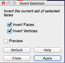
18. Select Filter>Selection>Invert Selection
    
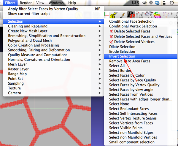
19. Apply the Inversion
    
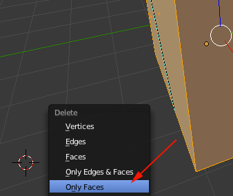
20. Click the Delete Faces button.
    
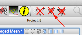
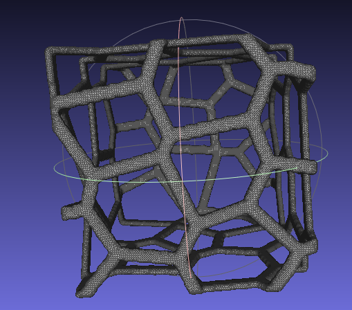
21. You should have a single-sided Voronoi mesh.
    
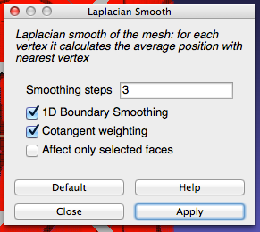
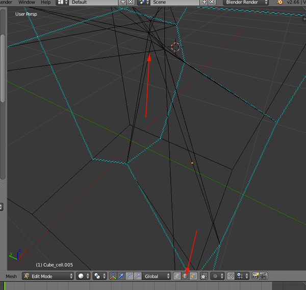
22. Time to refine the mesh. Select Filters>Smoothing, Fairing, and Deformation>Laplacian Smooth.
    
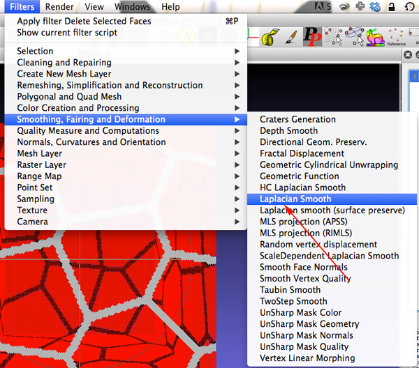
23. Apply the filter
    
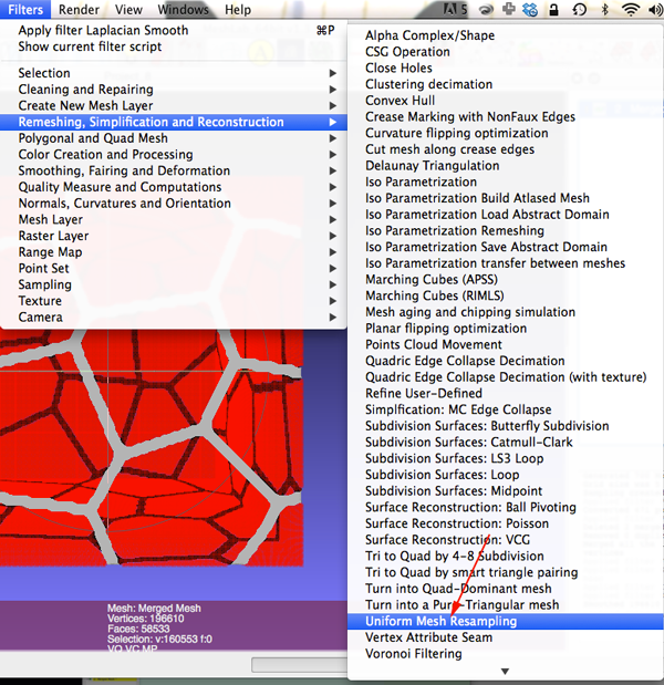
24. You still have just a 2D mesh. You need to extrude the mesh. Select Filters>Remeshing, Simplification, and Reconstruction>Uniform Surface Resampling
    
25. Make sure your dialog box looks similar
    
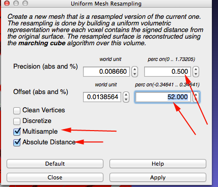
26. Click Apply. This will take some time to process. Be patient.
27. Turn off the layer that is not the offset layer./li>
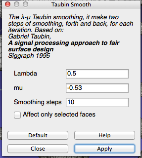
28. Select the Offset layer. One last smothing algorithm: select Filters>Smoothing, Fairing, and Deformation>Taubin Smooth.
    
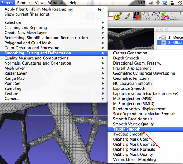
29. Keep the defaults and apply Taubin filter
    
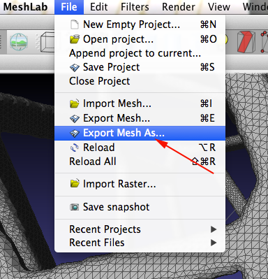
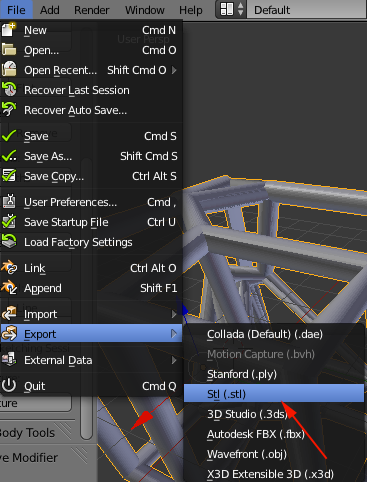
30. Export As and save as an STL
    

Analysis

1. Compare the different forms created. What is responsible for the similarities or differences?
2. Design a practical object that takes advantage of the voronoi algorithm
3. Explore creating Voronoi diagrams with other applications: TinkerCad and/or Blender

TinkerCad

TinkerCad has a Voronoi shape that can be found under Shape Generators To get a similar skeletal effect

1. Drag the shape on to the workplane.
2. Increase the Cell Spacing.
3. Convert the shape to a hole.
4. Drag a box on to the workplane and adjust the width, length and height so that the voronoi shape can be subtracted from the box
   
   

Blender

Version 1

1. Open Blender
2. If you have not turned on Cell Fracture
   1. Open User Preferences
      
   2. Click on the Addons
   3. Search for cell or just click on Objects and enable Cell Fracture
      
   4. Click Save User Settings
   5. Close User Preferences
3. Scale your cube to a reasonable printing size or delete it and import another model or add another mesh
4. Click on Cell Fracture
   
5. Go with the defaults or customize:
   
   
6. Click OK
7. Click on Layer 2
   
8. Click on one of the pieces and press A until all are selected
   
9. Press CTRL+J to combine all pieces
10. With the object selected navigate to Edit Mode
11. Enable Face Select
    
12. Select Vertices from Mesh menu and Remove Doubles. Also up the Merge Difference
    
13. Press A to deselect and then A to reselect all
14. Press X and Delete Only Faces
    
15. Select Edges and select all interior edges
    
    
16. Delete the selected edges
17. Ensure that all interior (black) edges are removed
    
18. Select Vertices
    
19. Select all Vertices by pressing A:
    
20. Select the Skin Modifier
    
21. Press CTRL+A to adjust thickness of mesh
    
22. Navigate to Object Mode (You must be in Object Mode to apply the modifier).
    
23. Apply the Skin Modifier
    
24. Apply a Subsurf Modifier
    
25. Under the File menu select Export and select STL
    

Version 2

1. Open Blender
2. If you have not turned on Cell Fracture
   1. Open User Preferences
      
   2. Click on the Addons
   3. Search for cell or just click on Objects and enable Cell Fracture
      
   4. Click Save User Settings
   5. Close User Preferences
3. Scale your cube to a reasonable printing size or delete it and import another model or add another mesh
4. Click on Cell Fracture
   
5. Go with the defaults or customize:
   
   
6. Click OK
7. Click on Layer 2
   
8. Click on one of the pieces and press A until all are selected
   
9. Press CTRL+J to combine all pieces
10. With the object selected navigate to Edit Mode
11. Enable Face Select
    
12. PressA to deselect and then A to reselect all
13. Press X and Delete Only Faces
    
14. Select Mesh>Vertices>Remove Doubles
    
15. Navigate back to Object Mode
16. Select Object>Convert to>Curve from Mesh/Text or press ALT+C
    
17. Press SHIFT+A and select curve>Circle
18. Resize the circle making it small. You can also press N for better control
    
19. Deselect the circle and select your model
    
20. On the right select Object Data
21. Under Bevel Object select the bezier curve. Select Fill Caps and Fill Deformed
    
22. Select Object>Convert to>Mesh from Curve or press ALT+C
23. Under the file menu select Export and select STL
    
24. Chances are you will not have an object that is manifold. Open in NetFabb to repair