OpenSCAD
Math
This tutorial will show you how OpenSCAD can use math.How do I make this?
- If you do not have OpenSCAD installed, download the application from openscad.org
- Download 3dplot.scad and place it in the same directory as your OpenSCAD file that will use it.
- Open 3dplot.scad and comment out all the examples. Save the file.
- Create a new OpenSCAD document. Save it as 2dgraphing.scad. This code is derived from
 user Brad Pitcher:
pi = 3.1415926536; e = 2.718281828; /************************* * Cartesian equations *************************/ /* Sine wave */ module sineWave(){ linear_extrude(height=5) 2dgraph([-50, 50], 3, steps=50); } module parabola (){ linear_extrude(height=5) 2dgraph([-50, 50], 3, steps=40); } /* Ellipsoid - use a cartesion equation for a half ellipse, then rotate extrude it */ module ellipsoid(){ rotate_extrude(convexity=10, $fn=100) rotate([0, 0, -90]) 2dgraph([-50, 50], 3, steps=100); } /************************* * Polar equations *************************/ /* Rose curve */ module rose(){ scale([20, 20, 20]) linear_extrude(height=0.15) 2dgraph([0, 720], 0.1, steps=160, polar=true); } /* Archimedes spiral */ module archimedesSpiral(){ scale([0.02, 0.02, 0.02]) linear_extrude(height=150) 2dgraph([0, 360*3], 50, steps=100, polar=true); } /* Golden spiral */ module goldenSpiral(){ linear_extrude(height=50) 2dgraph([0, 7*180], 1, steps=300, polar=true); } /************************** * Parametric equations *************************/ /* 9-pointed star */ module ninePointedStar(s,h){ scale(s) linear_extrude(height=h) 2dgraph([10, 1450], 0.1, steps=9, parametric=true); } /*************************/ // function to convert degrees to radians function d2r(theta) = theta*360/(2*pi); // These functions are here to help get the slope of each segment, and use that to find points for a correctly oriented polygon function diffx(x1, y1, x2, y2, th) = cos(atan((y2-y1)/(x2-x1)) + 90)*(th/2); function diffy(x1, y1, x2, y2, th) = sin(atan((y2-y1)/(x2-x1)) + 90)*(th/2); function point1(x1, y1, x2, y2, th) = [x1-diffx(x1, y1, x2, y2, th), y1-diffy(x1, y1, x2, y2, th)]; function point2(x1, y1, x2, y2, th) = [x2-diffx(x1, y1, x2, y2, th), y2-diffy(x1, y1, x2, y2, th)]; function point3(x1, y1, x2, y2, th) = [x2+diffx(x1, y1, x2, y2, th), y2+diffy(x1, y1, x2, y2, th)]; function point4(x1, y1, x2, y2, th) = [x1+diffx(x1, y1, x2, y2, th), y1+diffy(x1, y1, x2, y2, th)]; function polarX(theta) = cos(theta)*r(theta); function polarY(theta) = sin(theta)*r(theta); module nextPolygon(x1, y1, x2, y2, x3, y3, th) { if((x2 > x1 && x2-diffx(x2, y2, x3, y3, th) < x2-diffx(x1, y1, x2, y2, th) || (x2 <= x1 && x2-diffx(x2, y2, x3, y3, th) > x2-diffx(x1, y1, x2, y2, th)))) { polygon( points = [ point1(x1, y1, x2, y2, th), point2(x1, y1, x2, y2, th), // This point connects this segment to the next point4(x2, y2, x3, y3, th), point3(x1, y1, x2, y2, th), point4(x1, y1, x2, y2, th) ], paths = [[0,1,2,3,4]] ); } else if((x2 > x1 && x2-diffx(x2, y2, x3, y3, th) > x2-diffx(x1, y1, x2, y2, th) || (x2 <= x1 && x2-diffx(x2, y2, x3, y3, th) < x2-diffx(x1, y1, x2, y2, th)))) { polygon( points = [ point1(x1, y1, x2, y2, th), point2(x1, y1, x2, y2, th), // This point connects this segment to the next point1(x2, y2, x3, y3, th), point3(x1, y1, x2, y2, th), point4(x1, y1, x2, y2, th) ], paths = [[0,1,2,3,4]] ); } else { polygon( points = [ point1(x1, y1, x2, y2, th), point2(x1, y1, x2, y2, th), point3(x1, y1, x2, y2, th), point4(x1, y1, x2, y2, th) ], paths = [[0,1,2,3]] ); } } module 2dgraph(bounds=[-10,10], th=2, steps=10, polar=false, parametric=false) { step = (bounds[1]-bounds[0])/steps; union() { for(i = [bounds[0]:step:bounds[1]-step]) { if(polar) { nextPolygon(polarX(i), polarY(i), polarX(i+step), polarY(i+step), polarX(i+2*step), polarY(i+2*step), th); } else if(parametric) { nextPolygon(x(i), y(i), x(i+step), y(i+step), x(i+2*step), y(i+2*step), th); } else { nextPolygon(i, f(i), i+step, f(i+step), i+2*step, f(i+2*step), th); } } } } - Open another OpenSCAD document.
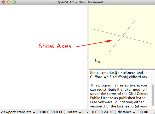
- To display the axes in the model view press Command+2 (MAC) or CTRL+2 (Windows and Linux).

- Save the new document as openscadMath.scad in the same place as you saved 2dgraphing.scad.
- The first line of the new file should be :
include <2dgraph.scad>
include <3dplot.scad>
- This is how you would create a sine wave:
Press F5 to render
function _f(x) = 20*sin((1/4)*x);
function f(x) = _f(d2r(x));
sineWave();
- Here are some other shapes:
Shape Code Parabola function f(x) = pow(x, 2)/20; parabola();
ellipsoid function f(x) = sqrt((2500-pow(x, 2))/3); ellipsoid();
rose function r(theta) = cos(4*theta); rose();
Archimedes Spiral function r(theta) = theta/2*pi; archimedesSpiral();
Golden Spiral function r(theta) = pow(e, 0.0053468*theta); goldenSpiral();
Nine Pointed Star function x(t) = cos(t); function y(t) = sin(t); ninePointedStar([10,10,10],0.25);
- For the 3d graphing there are four example graphs to play with:
Select one or two, uncomment them and render the 3D graph (F5)Graph Code Square ripples in a pond function z(x,y) = 2*cos(rad2deg(abs(x)+abs(y))); 3dplot([-4*pi,4*pi],[-4*pi,4*pi],[50,50],-2.5);
A wash board function z(x,y) = cos(rad2deg(abs(x)+abs(y))); 3dplot([-4*pi,4*pi],[-4*pi-20,4*pi-20],[50,50],-1.1);
Uniform bumps and dips function z(x,y) = 5*cos(rad2deg(x)) * sin(rad2deg(y)); 3dplot([-2*pi,2*pi],[-2*pi,2*pi],[50,50],-6);
sombrero function function z(x,y) = 15*cos(180*sqrt(x*x+y*y)/pi)/sqrt(2+x*x+y*y); 3dplot([-4*pi,+4*pi],[-4*pi,+4*pi],[50,50],-5);
- OpenSCAD also includes syntax for for loops. Here is an example that takes advantage of the cos() function:
for(i=[0:36]){
    for(j=[0:10]){
        translate([i*10,j*10,0])cylinder(r=5,h=cos(i*10)*50+60);
    }
}
- Here is an example that takes advantage of the sin() function:
for(i=[0:36]){
    for(j=[0:10]){
        translate([i*10,j*10,0])cylinder(r=5,h=sin(i*10)*50+60);
    }
}
- Create an interesting math form
Why am I doing this?
OpenSCAD allows you to generate interesting forms by taking advantage of math. This tutorial also demonstrated how to reuse modules across files.
Now what?
- Upload your math form to Thingiverse
- Come back tomorrow for more information and inspiration!
